Python Scriptと一緒に理解するCNN（Convolutional Neural Networks）の仕組み Conv2D編
How CNN (Convolutional Neural Networks) Works with Python Scripts ~ Conv2D ~

画像認識シリーズ第7弾です。前回のブログ記事。

This is the 7th image recognition series. Last blog post.

前回は全体コードの概要とmain関数内の図による説明をおこないました。

In a previous blog post, I outlined the entire code and explained the [main function] with diagrams.

この手のものはやり尽くされていますが、ただ一から全部やってみたかった。それだけです。 つーことでお次は前回のPythonスクリプトが実際にどのようにCNNを構築しているのかを解説していきたいと思いMASU。

This kind of thing is done by many people, but I just wanted to do it all from scratch. That's all. Next, I'll show you how the previous Python script actually built CNN, and how it works.

前回はmain関数内まで図を用いた説明を行ったので、その続き。 ２つの関数とそれに伴うCNNの基本的な考えを図を用いて説明したいでごわす。

The last time, I explained the main function with diagrams, and so on. I'd like to illstrate the tow functions and basic idea behind CNN with diagrams.

取り敢えず全体のコードは以下になります。

For now, the whole script is as follows.

Improved version of cifar10_cnn.py

imp_ver_cf10cnn.py

import keras
from keras.models import Sequential
from keras.layers import Dense, Dropout, Activation, Flatten
from keras.layers import Conv2D, MaxPooling2D
from keras.utils import np_utils
import numpy as np


labels = ["dogs", "cats", "monkeys", "birds", "fish", "lizards"]
total_num = len(labels)
image_size = 100

batch_size = 32
epochs = 100

def main():
  X_train, x_test, Y_train, y_test = np.load("data/augumented_images.npy")
  X_train = X_train.astype("float") / 256
  x_test = x_test.astype("float") / 256
  Y_train = np_utils.to_categorical(Y_train, total_num)
  y_test = np_utils.to_categorical(y_test, total_num)

  model = model_train(X_train, Y_train)
  model_eval(model, x_test, y_test)

def model_train(X, y):
  model = Sequential()
  model.add(Conv2D(32, (3, 3), padding='same',
                  input_shape=X.shape[1:]))
  model.add(Activation('relu'))
  model.add(Conv2D(32, (3, 3)))
  model.add(Activation('relu'))
  model.add(MaxPooling2D(pool_size=(2, 2)))
  model.add(Dropout(0.25))

  model.add(Conv2D(64, (3, 3), padding='same'))
  model.add(Activation('relu'))
  model.add(Conv2D(64, (3, 3)))
  model.add(Activation('relu'))
  model.add(MaxPooling2D(pool_size=(2, 2)))
  model.add(Dropout(0.25))

  model.add(Flatten())
  model.add(Dense(512))
  model.add(Activation('relu'))
  model.add(Dropout(0.5))
  model.add(Dense(total_num))
  model.add(Activation('softmax'))

  opt = keras.optimizers.adam()

  model.compile(loss='categorical_crossentropy',
              optimizer=opt,
              metrics=['accuracy'])
  
  model.fit(X,y,batch_size=batch_size, epochs=epochs)

  model.save("data/creatures_cnn.h5")

  return model

def model_eval(model, X, y):
  scores = model.evaluate(X, y, verbose=1)
  print('Test Loss', scores[0])
  print('Test Accuracy', scores[1])

if __name__=="__main__":
  main()

main()内の説明は前回で終わったので、今回は２つの関数、model_trainとmodel_evalの説明をしていきたいDESU。

In the previous blog post, I finished the explain for the main function. In this blog post, I will describe two function, model_train and model_eval with diagrams.

まず最初にモデルを作る準備をします。

First, we prepare to make a learning model.

model = Sequential()

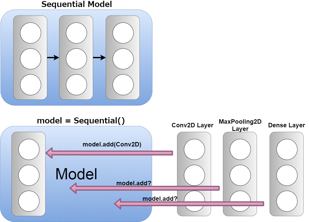
モデルは今の段階ではただの箱です。 この空箱に、レイヤーと呼ばれる、ある特定の働きをするデータの集まりを、継ぎ足していけるようにします。 このレイヤー同士は「Sequentialな」（順番に次々と）繋がなっている状態になります。

The model is just a box at this stage. This empty box can be filled with layers of a collection of data that serves a particular function. The layers are "Sequential" connected.

続いてこちらのコード。

Next, I'll explain the following code.

model.add(Conv2D(32, (3, 3), padding='same', input_shape=X.shape[1:]))

Conv2dは２d（二次元情報）（今みんなが見ているディスプレイも二次元情報です） の畳み込みを行うレイヤーを作成する。 この場合画像一枚（100ピクセル×100ピクセル）（100マス×100マスの正方形）に対して、 （３ピクセル×３ピクセル）（３マス×３マス）の正方形を作り、 それをスライドさせて、畳み掛けるようにこの画像のピクセル情報に フィルター（この画像における特徴一つを抽出して、そのピクセル数値を順次掛け合わせていく）をかけていく。

図では６×６の白黒画像に、画像の一部分を切り取った２x２の特徴１で説明している。

Conv2d is 2d (two-dimensional infomaition) (The display that people are looking at now is also two-dimensional infromation) creates a convolutional layer. In this case, for one image (100 pixels by 100 pixels) (100 squares by 100 squares), Make a square of (3 square by 3 square) (3 pixels by 3 pixels) then slide it around, and apply a filter (One feature in the image is extracted and the pixel values are multiplied sequentially).

In the figure, a black and white image of 6 by 6 is described with the feature 1 of 2 by 2 obtained by cutting a part of the iamge.

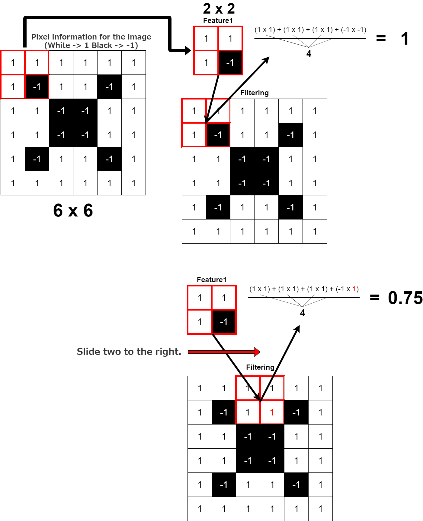
同じ特徴なら「１」が計算され、次の特徴なら「0.75」ポイント。比べた特徴同士がどれくらい似ているかの指標になる。

If it is the same shape, it is caculated as 1. If it is the next shape, it is [0.75] point. It is an indicator of how similar the shapes are.

Conv2D(5, (2, 2)

試しにこのようなConv2Dレイヤーを作るとどうなるか。

What happens when you try to create a Conv2D layer like this?

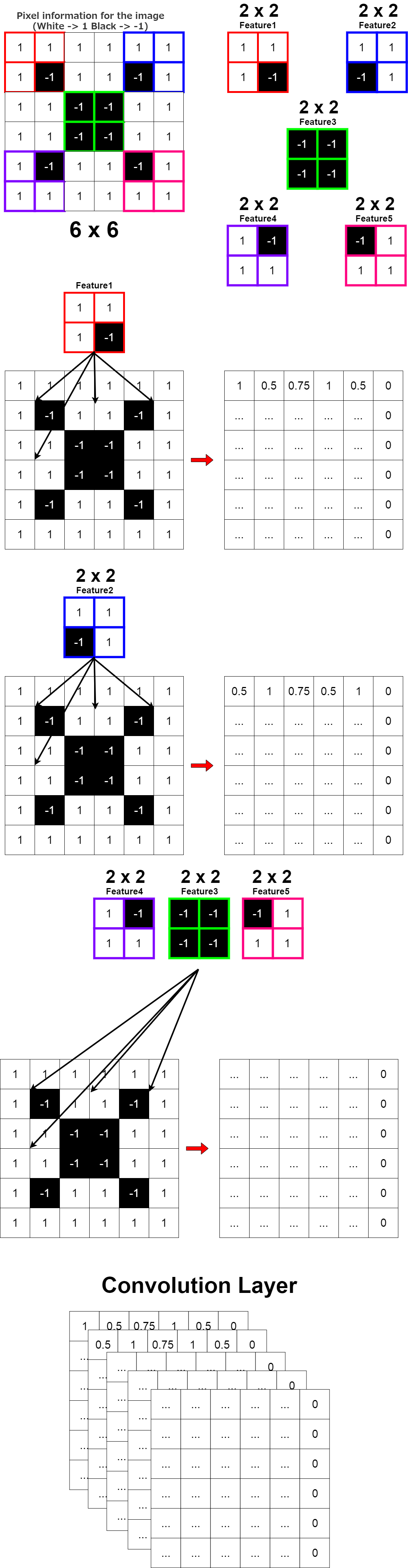
model.add(Conv2D(32, (3, 3), padding='same', input_shape=X.shape[1:]))

つまり、画像一枚につき、合計32枚の画像をフィルターしたものができる。 そして引数のpadding＝”same”は入力した画像のサイズと出力サイズ（フィルターをかけた後のサイズ）を一緒にするという意味。 数を合わせる為に端を「０」で埋める（パディング）するのでPaddingという引数名になる。

That is, each image can be filtered for a total of 32 times. The argument [padding="same"] means that the input image size and the output size (Size after filtering) are the same. Fill the ends with [0] to match the pixels of input image. (zero padding)

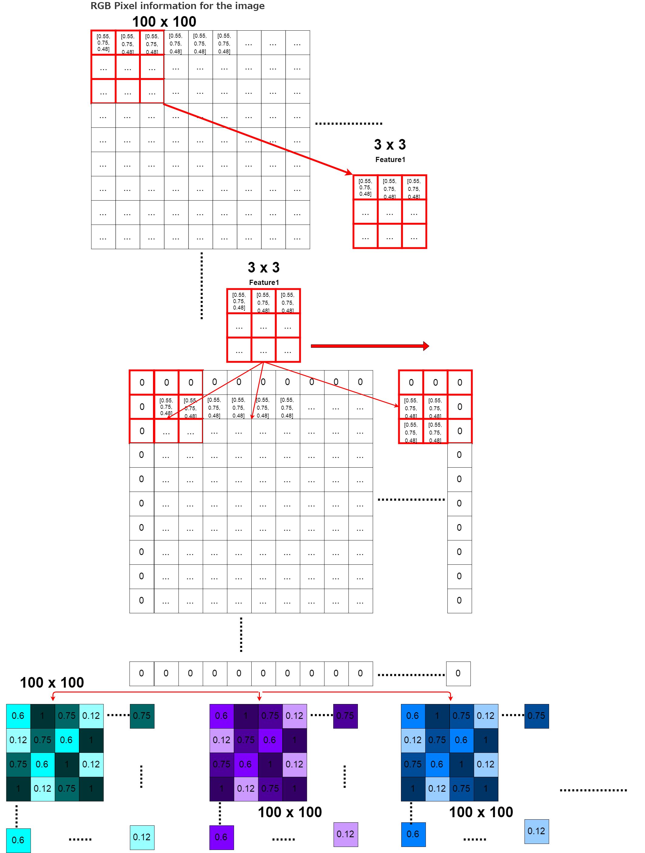
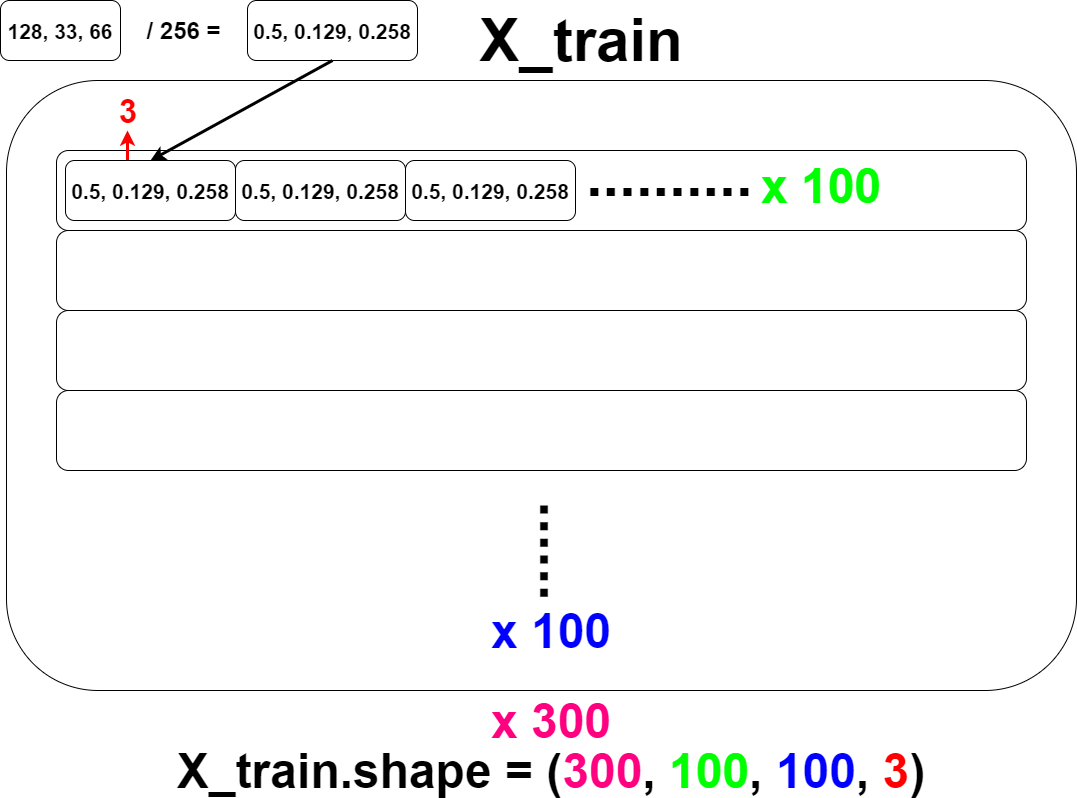
最後、「input_shape=X.shape[1:]」ですが、X.shape[1:]を使う、つまり訓練データのNumpy配列形状の一番目以降を使うという意味です。 この場合この関数に渡される引数の「X」はX_train、つまり訓練用の画像データです。 numpyではX_train.shapeとすると、例えば「３００、１００、１００、３」といった具合に ３00枚の画像情報が、100行100列、各行あたり３個の（RGB情報）で、構成されてますと表示されます。 この「３００、１００、１００、３」の「１００、１００、３」の部分だけ使います。

And finally, the description of [input_shape=X.shape[1:]]. In this case, the "X" in the argument passed to the function is X_train, the training image data. if you run [X_train.shape], you will see something like [300, 100, 100, 3]. This means that there are a matrix of 100 rows and 100 columns with 3 pieces of pixels information (RGB) per row in 300 pieces of image data. Only the [100, 100, 3] part of this [300, 100, 100, 3] is used.

長くなってしまったので、残りの説明は次回に持ち越します。お次は活性化関数”ReLU”からです。

As it has become too long, I will carry over the rest of the explanation next time. Next comes the activation function [ReLU].

See You Next Page!