Python Scriptと一緒に理解するCNN（Convolutional Neural Networks）の仕組み 勾配法編
How CNN (Convolutional Neural Networks) Works with Python Scripts ~ Gradient method ~

画像認識シリーズ第17弾です。前回のブログ記事。

This is the 17th image recognition series. Last blog post.

前回は勾配の図による説明をおこないました。

In a previous my blog post, I explained the gradient along with diagrams.

今回の記事は最適化において重要な勾配法についての説明をしていきます。

In this blog post, I'm going to briefly talk about gradient method which is important in optimization.

この手のものはやり尽くされていますが、ただ一から全部やってみたかった。それだけです。 つーことで今回は勾配法に関してを解説していきたいと思いMASU。

This kind of thing is done by many people, but I just wanted to do it all from scratch. That's all. Anyway, I would like to explain about gradient method this time.

今回のような損失値の最小値を探すような場合は勾配法の一つ、勾配降下法を使います。

If you want to find the minimum value of the loss value like this time, use the gradient descent method, which is one of the gradient methods.

前回の趣旨で説明した通り、勾配降下法は谷のような場所の一番深い部分を探す方法です。

As I explained in the previous blog post, the gradient descent method is a way to find the deepest part of a place like a valley.

この図の様な単純な斜面からボールを転がすことを想像してください。

Imagine rolling a ball down a simple slope like this.

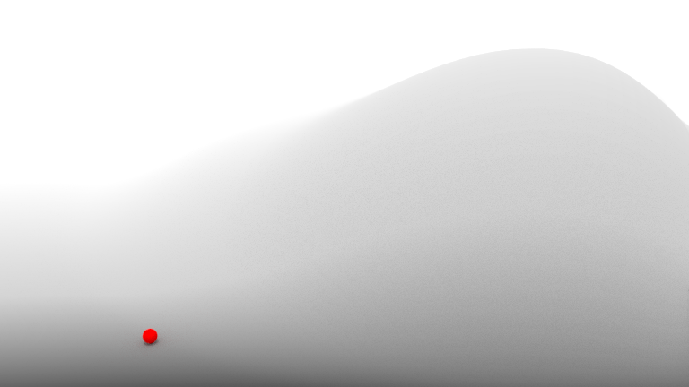
ボールは重力に従って急斜面を転がって、やがてなだらかな場所に落ち着きます。

The ball rolls down a steep slope in accordance with gravity, eventually settling on a flat surface.

勾配降下法の仕組みは大体この通りです。

The mechansim of the gradient descent method is roughly like this.

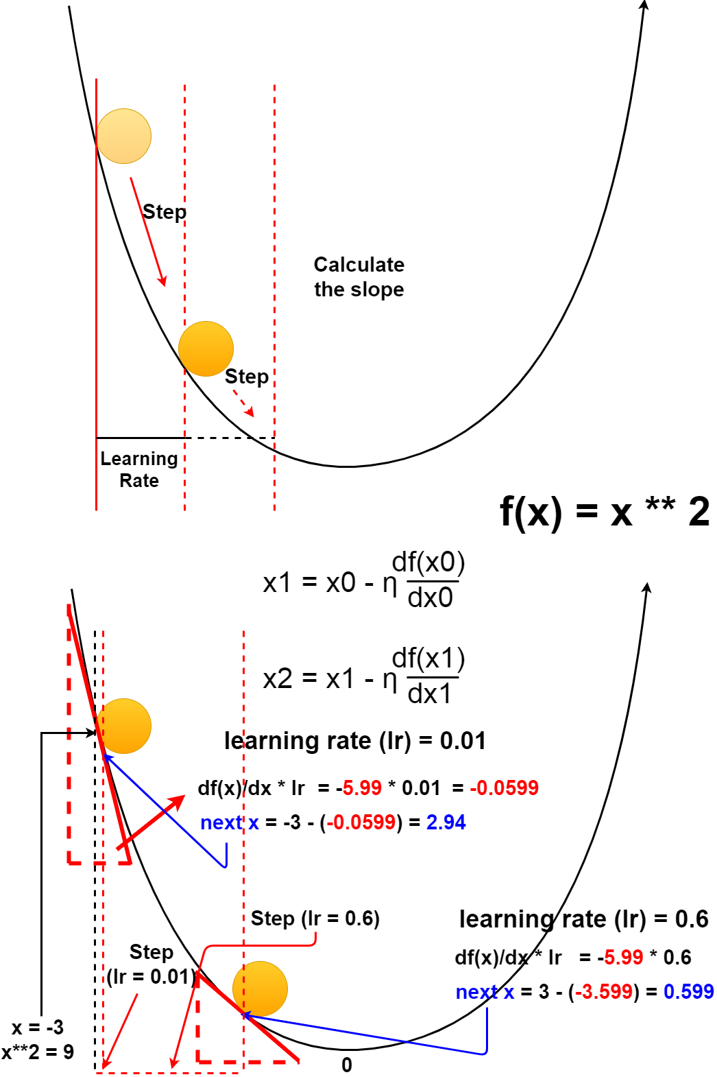
図にするとスムーズに移動しているように見えますが、 実はこのボールは、一歩ずつ斜面を計算して、それを繰り返して進んでいます。

It looks like it's moving smoothly in the diagram, but in fact, the ball is calculating the slope step by step and repeating it.

その一歩の歩幅は学習率（ηイータ）という値で設定します。

The step length is set as the learning rate η (eta).

ちょっと分かりにくいですが、数式と考え方は図の通りです。

It's a little hard to understand, but the formula and idea are as shown in the diagram.

Pythonコードで試してみましょう。

Let's try it in Python scripts

import numpy as np

def func1(x):
    return x**2 + 1

def func2(params):
    return np.sum(np.power(params,2))

def differentiation(f, x):
    h = 1e-7
    return (f(x + h) - f(x - h)) / (2*h)

def gradient(f, params):
    h = 1e-7
    grad = np.zeros_like(params)
    for idx in range(params.size):
        tmp_val = params[idx]
        params[idx] = tmp_val + h
        fxh1 = f(params)
        params[idx] = tmp_val - h
        fxh2 = f(params)
        grad[idx] = (fxh1 - fxh2) / (2*h)
        params[idx] = tmp_val
    return grad

def desc_meth(f, init_x, lr=0.01, step=100):
    x = init_x
    for i in range(step):
        slope = differentiation(f, x)
        x -= lr * slope
    return x

def grad_desc_meth(f, init_params, lr=0.01, step=100):
    params = init_params
    for i in range(step):
        grad = gradient(f, params)
        params -= lr * grad
    return params

学習率が小さいと（Step数が多くなり）時間がかかります。

If the learning rate low (as the number of steps increases), you can be time consuming.

init_x = -3.0

# learning rate 0.01 step 500
In : desc_meth(func1, init_x, lr=0.01, step=500)
Out: -0.00012307192187321903

# learning rate 0.001 step 5000
In : desc_meth(func1, init_x, lr=0.001, step=5000)
Out: -0.00013484277838493597

学習率が大きくても学習に時間がかかります。

Learning takes time if the learning rate is high.

# learning rate 0.999 step 5000
In : desc_meth(func1, init_x, lr=0.999, step=5000)
Out: -0.00013485598670825993

学習率が極端に小さすぎたり、大きすぎたりすると更新が行われないか、値が発散して学習ができなくなります。

If the learning rate is too small or too large, no updates occur, or values diverge, preventing learning.

# If the learning rate is too small

# learning rate 1e-9(0.000000009) step 100
In : desc_meth(func1, init_x, lr=1e-9, step=100)
Out: -2.99999940000006

# learning rate 1e-9(0.000000009) step 1000
In : desc_meth(func1, init_x, lr=1e-9, step=100)
Out: -2.9999940000060055

# learning rate 1e-9(0.000000009) step 10000
In : desc_meth(func1, init_x, lr=1e-9, step=100)
Out: -2.999940000600035

# If the learning rate is too large

# learning rate 10.0 step 100
In : desc_meth(func1, init_x, lr=10.0, step=100)
Out: 2459382288.1580424

# learning rate 10.0 step 1000
In : desc_meth(func1, init_x, lr=10.0, step=1000)
Out: 2459382288.1580424

ちなみに、学習率とStepはハイパーパラメータと言います。 要するに人が自分の手で入力しなければならない数値です。 反対にパラメータは学習アルゴリズムによって自動的に決まっていきます。 （今回は最初だけ手入力してますが、実際は全結合層にある重みやバイアス等がパラメータにあたります。）

By the way, learning rate and step are called hyperparameters. In short, it is a number that people have to input by themselves. In contrast, the parameters are determined automatically by the learning algorithm. (This time, we manually input the parameters only at the beginning, but actually, the parameters are the weights and biases of all in the fully connected layers.)

では次に複数の変数からなる関数で勾配降下法を試してみます。

Now let's try the gradient decsent method with a multi-variable function.

init_params = np.array([3.0, 3.0])

# learning rate 0.01
In : grad_desc_meth(func2, init_params=init_params, lr=0.01, step=100)
Out: array([0.39785867, 0.39785867])

# learning rate 0.1
In : grad_desc_meth(func2, init_params=init_params, lr=0.1, step=100)
Out: array([8.1045242e-11, 8.1045242e-11])

# learning rate 0.0001
In : grad_desc_meth(func2, init_params=init_params, lr=0.0001, step=100)
Out: array([7.94402798e-11, 7.94402798e-11])

# learning rate 0.01 step 1000
In : grad_desc_meth(func2, init_params=init_params, lr=0.01, step=1000)
Out: array([1.33695391e-19, 1.33695391e-19])

init_params = np.array([3.0, 6.0, 9.0])

# learning rate 0.01 step 100
In : grad_desc_meth(func2, init_params=init_params, lr=0.01, step=100)
Out: array([6.69583151e-10, 1.33916630e-09, 2.00874945e-09])

# learning rate 0.01 step 1000
In : grad_desc_meth(func2, init_params=init_params, lr=0.01, step=1000)
Out: array([5.04890208e-09, 1.00978041e-08, 1.51467062e-08])

このように勾配が0に近づくよう、パラメータを更新していくことによって学習を進めるのが勾配降下法になります。

Thus, the gradient descent method works by updating the parameters so that the gradient approaches almost 0.

損失値の勾配が0に近いということは、それだけ確からしい画像や文字の判定ができているということです。

In fact, the gradient of the loss value is approaching 0 means that the learning model is able to determine more reliable images or characters.

では損失値が描く勾配がこのような複雑なものだったらどうするか。

What if the gradient of the loss value is so complex?

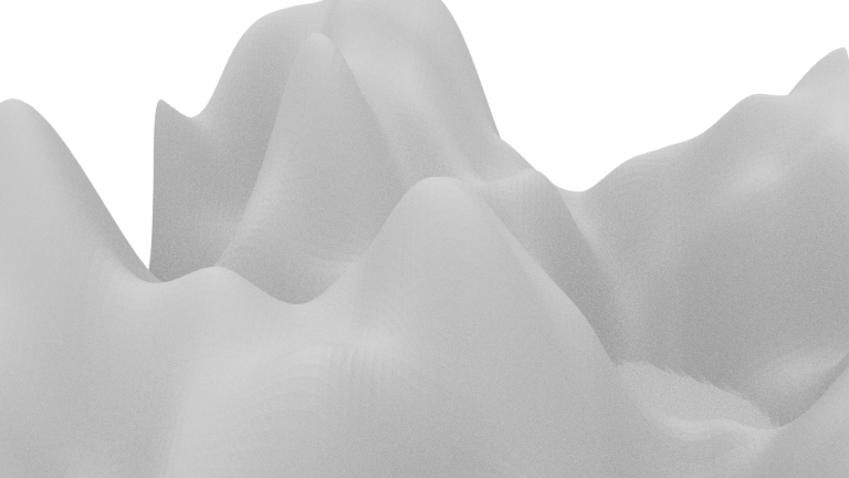
おどろおどろしい、幾つもの谷ができています。 ボールを落とす場所を間違えたら最も深い谷に辿り着く前に「すぽっと」エアーポケットのような場所でボールはストップしてしまいます。

There are many suspicious valleys. If you drop the ball at the wrong place, the ball stops at a place like an air pocket before reach the deepest area.

それを避けるには、ありとあらゆる場所からボールを落とす作業が必要になります。

To avoid that, you need to drop the ball from all over the place.

このように一つだけボールを落とす場所を決めるのではなく、複数のボールを無作為に選んで（パラメータの初期値）勾配法を適用する方法を確率的勾配法と言います。

In this way, the stochastic gradient descent is a method in which a plurality of balls (initial value of the parameter) are randomly selected and the gradient method is applied without limiting where the ball is dropped to only one place.

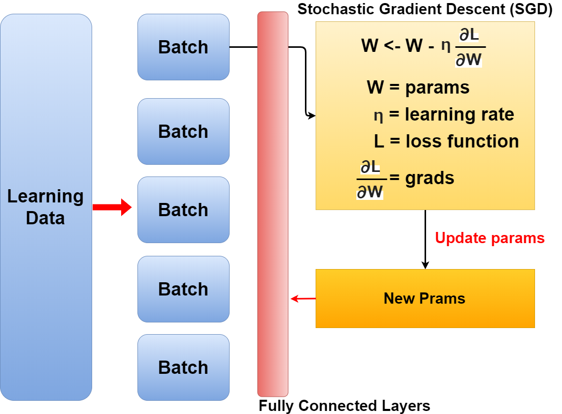
確率的勾配降下法(SGD)の手順は以下です。

The procedure for the stochastic gradient descent (SGD) is as follows.

• 其の１： 訓練データをバッチに分け、その中からランダムにデータを選び出す。

• Step 1： A plurality of pieces of data are randomly selected from the divided training data.

• 其の２： SGDを使い、損失関数の勾配を求める

• Step 2： Use SGD to find the gradient of the loss function for each weight.

• 其の３： 重みパラメーターの更新を行う。

• Step 3： The weight parameter is updated.

• 其の４： 手順１、２、３をエポックの数分繰り返す。

• Step 4： Repeat steps 1, 2 and 3, just the number of epochs.

残りの説明は次回に持ち越します。ということで、お次は最適化アルゴリズムについての説明DESU。ようやくですね。。。

I will carry over the rest of the explanation next time. So, In the next section, I'm going to illustrate about optimization algorithm. At last...

See You Next Page!