Python Scriptと一緒に理解するCNN（Convolutional Neural Networks）の仕組み 勾配編
How CNN (Convolutional Neural Networks) Works with Python Scripts ~ gradient ~

画像認識シリーズ第16弾です。前回のブログ記事。

This is the 16th image recognition series. Last blog post.

前回は誤差逆伝播法の基本、微分の図による説明をおこないました。

In a previous my blog post, I explained the differentiation which is the basics of the backpropagation along with diagrams.

今回の記事は最適化において重要な逆伝播誤差法、その中で使われている勾配についての説明をしていきます。

In this blog post, I'm going to briefly talk about gradient that used in "Backpropagation" which is important in optimization.

この手のものはやり尽くされていますが、ただ一から全部やってみたかった。それだけです。 つーことで今回は逆伝播誤差法、その中で使われている勾配に関してを解説していきたいと思いMASU。

This kind of thing is done by many people, but I just wanted to do it all from scratch. That's all. Anyway, I would like to explain about gradient that used in "Backpropagation" this time.

勾配の趣旨です。 勾配は次回説明する勾配法として使われる大事な要素です。

The purpose of the gradient described here. The gradient is an important element that is used as the gradient method, which I will illustrate in my next blog post.

その勾配法についての簡単な説明をしておきます。

I'll briefly describe the gradient method in this section.

簡単に一言で説明すると、勾配法は最適な重みなどのパラメーターを見つける為に行います。

In a nutshell, the gradient method is used to find the optimal weights and other parameters.

損失値が最小値を取る時に、最適なパラメータとなります。

The optimal parameter is the value of the parameter when the loss function takes the minimum value.

前回の大砲の弾道に対しての微分を、損失値が描く楕円に置き換えて考えてみてください。

In the previous article, we made a differentiate to the cannon trajectory, but this time consider replacing it with an ellipse drawn by the loss value.

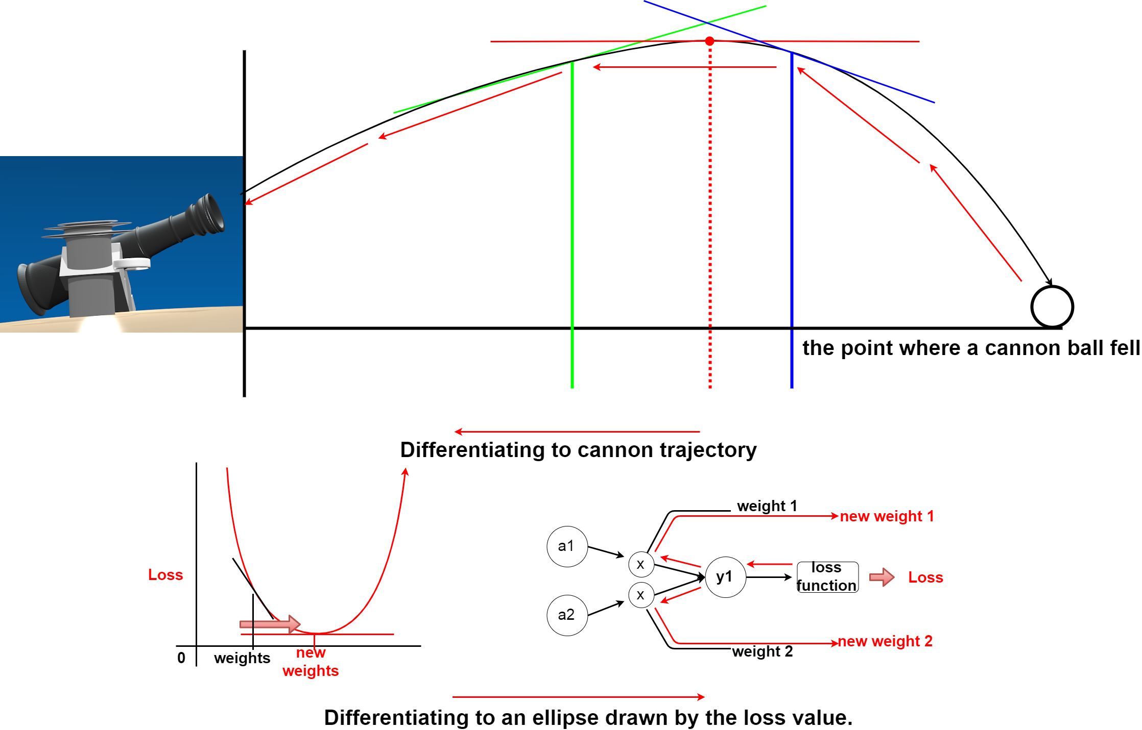
つまり、重み等のパラメータの値が少しだけ変化した場合の、損失関数が描く楕円の傾きが0になる場所（最小値）を探していくこができればいいわけです。

In other words, we need to find a place where the slope of the ellipse drawn by the loss function becomes 0 (Minimum) when the value of a parameter such as a weight changes slightly.

しかし、現実のパラメータの数は沢山あり、どれも損失値に影響しています。

However, there are many real parameters, all of which affect the loss value.

例えば512個のノードが、6個のノードに対してそれぞれ重みとなる値を掛けたとしたら。

Suppose, for example, that 512 nodes each multiplied 6 nodes by a weight value.

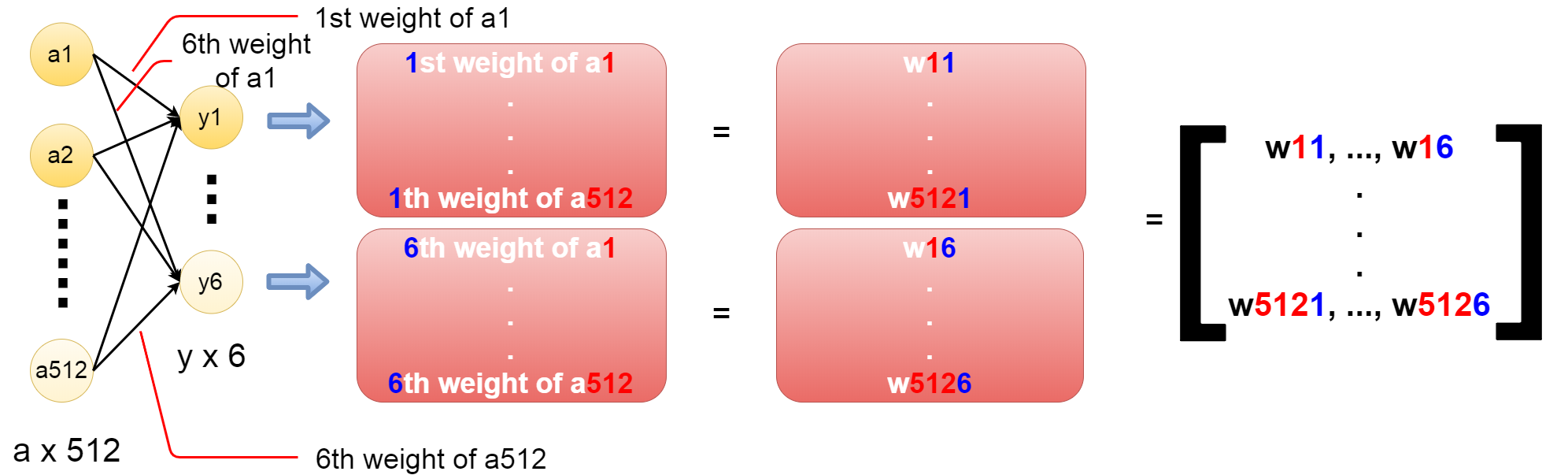
このようにパラメータ（変数）は複数あり、ベクトル化され、行列となる。

Thus, there are a plurality of parameters (variable), which are vectorized and represented as a matrix.

要は、複数の変数の関数を1つずつ微分するのではなく、それらを1つずつ微分して、ベクトルにまとめたものを勾配と呼び、 それを使って、損失値が最小の場所を探そうというのが勾配法です。

In other words, instead of differentiating the functions of multiple variables one by one, differentiate them at the same time and combining them into a vector is called a gradient. The gradient method is to find the place with the smallest loss value by using the gradient.

趣旨で説明した複数あるパラメーター（変数）を使った関数を、 まとめて微分したものを勾配と言います。

So, I explained previous section, gradient is instead of differentiating the functions of multiple variables one by one, differentiate them at the same time and combining them into as a vector.

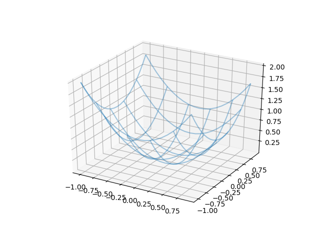
まず、２つの変数からなる関数があるとします。

First, suppose you have a function with two variables.

def func(x, y):
      return x ** 2 + y ** 2

そしてそれを３Dグラフにしてみます。

Then display the function as a 3D graph.

import numpy as np
import matplotlib.pyplot as plt
import mpl_toolkits.mplot3d.axes3d as axes3d

fig = plt.figure()
ax = fig.add_subplot(111, projection='3d')

x = np.arange(-1, 1, 0.01)
y = np.arange(-1, 1, 0.01)
X,Y = np.meshgrid(x, y)

Z = func(X,Y)

ax.plot_wireframe(X, Y, Z, rstride=4, cstride=4, alpha=0.4)

plt.show()

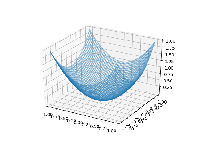
このグラフのXとYと関数が作る点に注目します。

In this graph, we assume that we have differentiated the curve produced by a function passing two variables, X and Y.

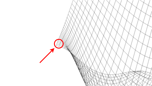
拡大します。

Zoom in.

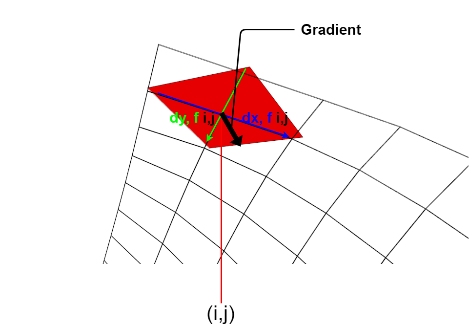
iとjはXとYの座標です。 ここからXの関数の微分とYの関数の微分を行い接面を作ります。

Where i and j are the X and Y coordinates. The derivative of the function X and the derivative of the function Y create the tangent surface to i and j.

図のように勾配はベクトルとして表現でき、 その接面において関数の値を最も減らす方向を指しています。

The gradient can be represented as a vector as shown in the diagram. It points in the direction where the value of the function decreases the most in the tangent surface.

ではこの勾配を別の図に直してみましょう。

Let's change this gradient to another diagram.

import numpy as np
import matplotlib.pyplot as plt
import mpl_toolkits.mplot3d.axes3d as axes3d

def func(x, y):
      return x ** 2 + y ** 2

fig = plt.figure()
ax = fig.add_subplot(111, projection='3d')

x = np.arange(-1, 1, 0.1)
y = np.arange(-1, 1, 0.1)
X,Y = np.meshgrid(x, y)

Z = func(X,Y)

ax.plot_wireframe(X, Y, Z, rstride=4, cstride=4, alpha=0.4)

plt.show()

上のスクリプトで図のようなグラフができます。

The above script draws a graph like this.

そしてそのまま下のスクリプトを実行すればベクトル表現された勾配の図ができます。

And if you just run the script below, you get a vector representation of the gradient.

def gradient(f, xy):
    h = 1e-7
    grad = np.zeros_like(xy)
    
    for i in range(xy.size):
        tmp_val = xy[i]
        xy[i] = float(tmp_val) + h
        fxh1 = f(xy[0], xy[1])
        
        xy[i] = tmp_val - h 
        fxh2 = f(xy[0], xy[1])
        grad[i] = (fxh1 - fxh2) / (2*h)
        
        x[i] = tmp_val
        
    return grad

X = X.flatten()
Y = Y.flatten()

XY = np.array([X, Y]).T

grad = np.zeros_like(XY)
    
for idx, xy in enumerate(XY):
    grad[idx] = gradient(func, xy)

grad = grad.T

plt.figure()
plt.quiver(X, Y, -grad[0], -grad[1],  angles="xy",color="blue")
plt.xlim([-1, 1])
plt.ylim([-1, 1])
plt.xlabel('x')
plt.ylabel('y')
plt.grid()
plt.draw()
plt.show()

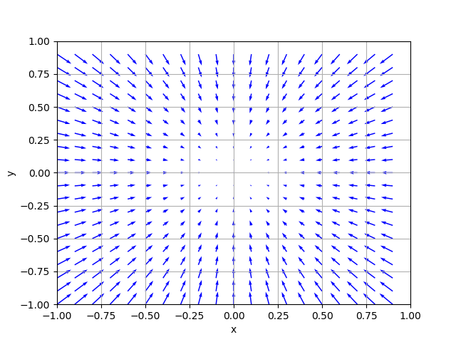
グラフの通り矢印の向きは斜面の方向、長さはどれだけ傾いているかを表しています。

As shown in the graph, the direction of the arrow represents the direction of the slope, and the length indicates how inclined the slope is.

後はこの矢印を辿って、勾配の先端まで行ったら、その地点からまた勾配を計算していきます。 それを繰り返していけば、最終的に斜面がなだらかになっている場所を見つけることができます。 これは勾配法のアルゴリズムの一つ、最急降下法と言われています。

Then, you follow this arrow to the tip of the slope and calculate the slope from that point. If you repeat it, you can finally find the place where the slope is smooth. This is called the Gradient descent method, which is one of the gradient method algorithms.

残りの説明は次回に持ち越します。お次は勾配を使った勾配法の具体例についての説明を予定してます。

I will carry over the rest of the explanation next time. Next, I'm going to explain of specific examples the gradient method by using the gradient.

See You Next Page!