Python Scriptと一緒に理解するCNN（Convolutional Neural Networks）の仕組み 全結合層 Flatten() Dense()編
How CNN (Convolutional Neural Networks) Works with Python Scripts ~ Fully Connected Layers Flatten() and Dense() ~

画像認識シリーズ第11弾です。前回のブログ記事。

This is the 11th image recognition series. Last blog post.

前回はmodel_train関数内のDropoutの図による説明をおこないました。

In a previous my blog post, I explained "Dropout", along with diagrams.

この手のものはやり尽くされていますが、ただ一から全部やってみたかった。それだけです。 つーことで今回は全結合層とFlatten()、Dense()に関してを解説していきたいと思いMASU。

This kind of thing is done by many people, but I just wanted to do it all from scratch. That's all. Anyway, I would like to explain about "Fully Connected Layers" and "Flatten(), Dense()" this time.

全結合層の簡単な概要です。 今までのConv2D、Activation、MaxPoolingの層を重ねた後に、 ニューラルネットワークを構築していきます。

A brief overview of Fully Connected Layers. After layering the previous Conv2D, Activation, and MaxPooling layers, We will build a neural network.

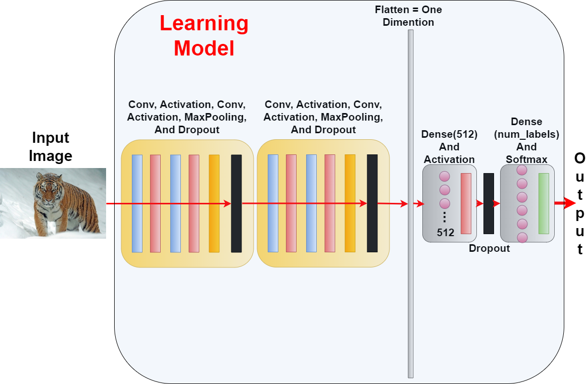
さらに上の図の全結合層の部分だけを模式図にすると以下にな〜る。

A schematic diagram of only the part [Fully Connected Layers] in the upper figure is as follows.

まずFlatten()から見ていきましょう

Let's start with "Flatten Function"

取り敢えず全体のコードは以下になります。

For now, the whole script is as follows.

Improved version of cifar10_cnn.py

imp_ver_cf10cnn.py

import keras
from keras.models import Sequential
from keras.layers import Dense, Dropout, Activation, Flatten
from keras.layers import Conv2D, MaxPooling2D
from keras.utils import np_utils
import numpy as np


labels = ["dogs", "cats", "monkeys", "birds", "fish", "lizards"]
total_num = len(labels)
image_size = 100

batch_size = 32
epochs = 100

def main():
    X_train, x_test, Y_train, y_test = np.load("data/augumented_images.npy")
    X_train = X_train.astype("float") / 256
    x_test = x_test.astype("float") / 256
    Y_train = np_utils.to_categorical(Y_train, total_num)
    y_test = np_utils.to_categorical(y_test, total_num)

    model = model_train(X_train, Y_train)
    model_eval(model, x_test, y_test)

def model_train(X, y):
    model = Sequential()
    model.add(Conv2D(32, (3, 3), padding='same',
                    input_shape=X.shape[1:]))
    model.add(Activation('relu'))
    model.add(Conv2D(32, (3, 3)))
    model.add(Activation('relu'))
    model.add(MaxPooling2D(pool_size=(2, 2)))
    model.add(Dropout(0.25))

    model.add(Conv2D(64, (3, 3), padding='same'))
    model.add(Activation('relu'))
    model.add(Conv2D(64, (3, 3)))
    model.add(Activation('relu'))
    model.add(MaxPooling2D(pool_size=(2, 2)))
    model.add(Dropout(0.25))

    model.add(Flatten())
    model.add(Dense(512))
    model.add(Activation('relu'))
    model.add(Dropout(0.5))
    model.add(Dense(total_num))
    model.add(Activation('softmax'))

    opt = keras.optimizers.adam()

    model.compile(loss='categorical_crossentropy',
                optimizer=opt,
                metrics=['accuracy'])
    
    model.fit(X,y,batch_size=batch_size, epochs=epochs)

    model.save("data/creatures_cnn.h5")

    return model

def model_eval(model, X, y):
    scores = model.evaluate(X, y, verbose=1)
    print('Test Loss', scores[0])
    print('Test Accuracy', scores[1])

if __name__=="__main__":
    main()

Flatten()がどのような働きをしているのか図でみませう。

Let's check how Flatten Function works with a diagram.

model.add(Flatten())

おっと間違えました。おふざけでつ。気にしないでね。忘れてくだちぃ。

Oops, I made a mistake. This is a different image. Next diagram is correct. Sorry about that. Just kidding...

model.add(Flatten())

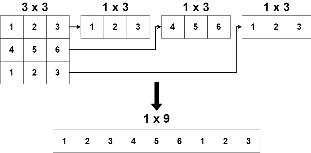
下の図では「３X３」のつまり「3行3列」の行列があります。 Flattenは単純にこの「３x３」の行列を「１x９」のベクトルにします。 「３x３」で全ての数値は「９つ」。 1次元のベクトルにする流れは上から順に「一行目」の方向の一番最後に「二行目」の頭をくっつける。 そして、「一行目と二行目がくっついたベクトル」の方向の一番最後に「三行目」の頭をくっつける。 とこんな感じどぅえす。

In the figure below, there is a 3 rows 3 columns matrix. Flatten simply makes this 3 x 3 matrix to 1 x 9 (one-dimensional) vector. 3 x 3 and all numbers are 9. In order to make a one-dimensional vector, the second row head is attached to the end of the first row. Then, the head of third row is attached to the end of the vector that are joined by the first and second row. It looks like this.

Flattenによって作られた一次元ベクトルを512個のノードに繋げてみましょう。

Now, let's connect the one-dimensional vector created by Flatten() one by one to 512 nodes using Dense().

model.add(Flatten())
model.add(Dense(512))

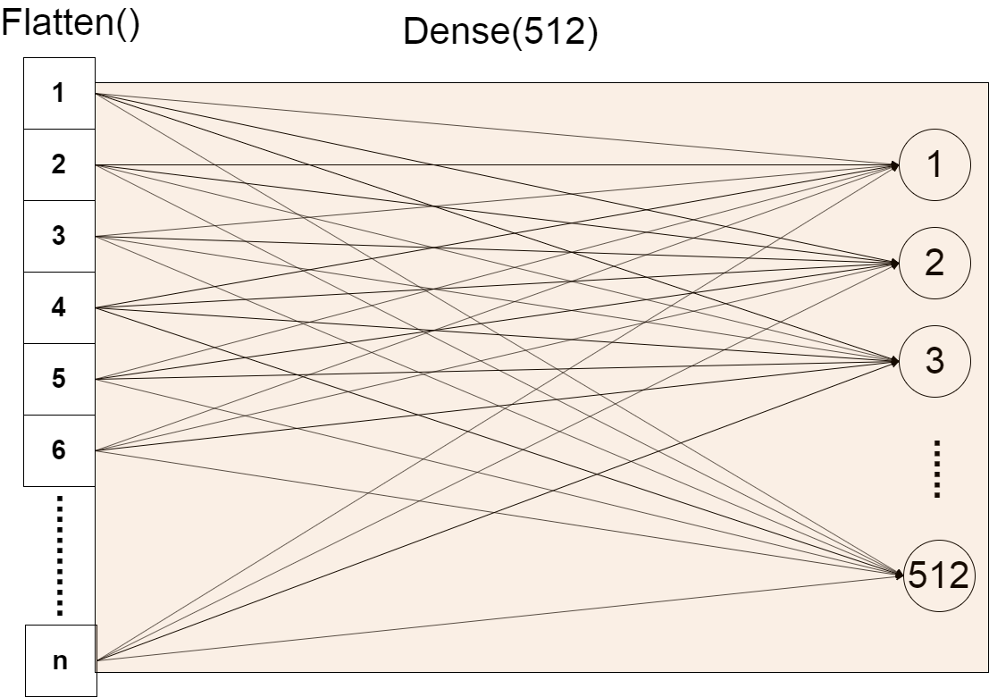
Dense(512)によって、512のノードにFlatten()が作ったベクトルの情報が伝達されるようになった。

By pssing 512 as an argument to Dense(), the vector information created by Flatten() is passed to the 512 nodes.

そして、その一つ一つのノードはベクトルの全ての数値に繋がっていることになる。

And each node is connected to all the values of the vector created by Flatten().

これが全結合です。

Thats the Fully Connected.

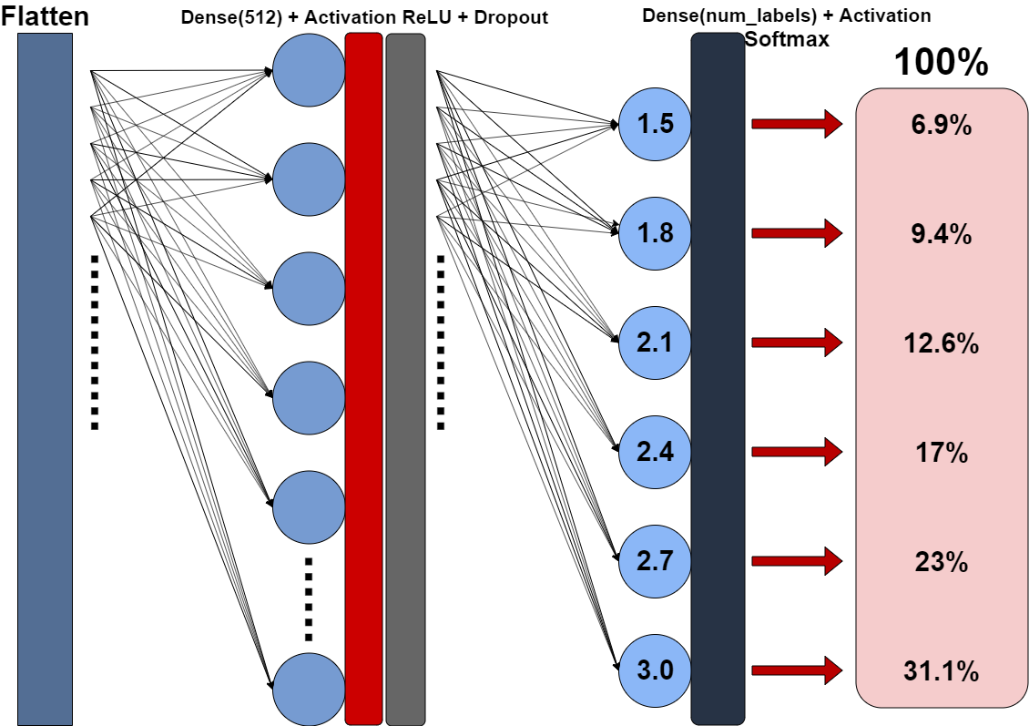
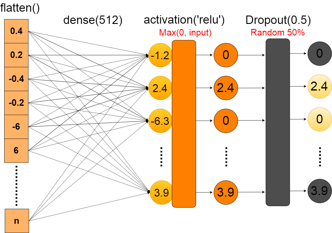
今までの関数をまとめて図で表示します。

I'll show you previous functions together in a diagram.

model.add(Flatten())
model.add(Dense(512))
model.add(Activation('relu'))
model.add(Dropout(0.5))

そして、ラベルの数だけのノードにまた全結合させます。

It then connectes all of the output from the Dropout function to the same number of nodes as the label.

model.add(Flatten())
model.add(Dense(512))
model.add(Activation('relu'))
model.add(Dropout(0.5))
model.add(number of labels)

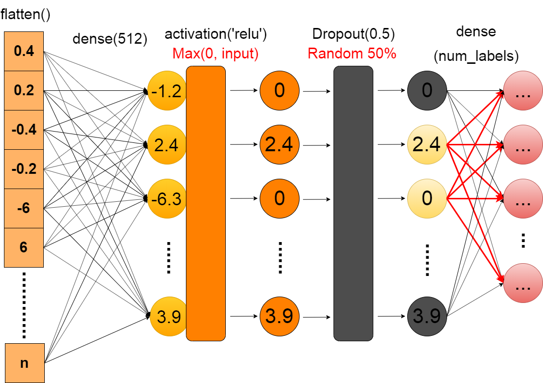
まとめると、Flatten()で入力する値を1次元のベクトルにして、 Dense()で指定したノードの数に「全結合」します。 活性化関数を用いて、非線形な値に変換します。 そして、Dropout()を50％に設定して、半分の出力をランダムに遮断して、 さらにそれらの出力をDense()によってラベルの数（今回は「猫、犬、鳥、猿、魚、トカゲ」の全6種類）だけ「全結合」します。

In summary, flatten() is used to make the values created by the Convolution layer into one-dimensional. It then uses dense() to "Fully Connected" the vector to the specified number of nodes. Then, it's converted into a nonlinear value using an activation function. Next, Set dropout() to 50% (0.5) to randomly block half of the output. Finally, Dense(num_labels) fully connects each value in the previous output by the specified number of labels. (This time, there are 6 types of "cats","dogs","birds","monkeys","fish", and "lizards", so there are 6 nodes.)

残りの説明は次回に持ち越します。お次はActivation('softmax')の説明を予定してます。

I will carry over the rest of the explanation next time. Next comes about Activation('softmax').

See You Next Page!