Published Date : 2019年11月24日21:02
Python Scriptと一緒に理解するCNN(Convolutional Neural Networks)の仕組み 最適化 逆伝播誤差法 微分編
How CNN (Convolutional Neural Networks) Works with Python Scripts ~ Optimizer Back propagation "Differentiation" ~
This blog has an English translation
画像認識シリーズ第15弾です。前回のブログ記事。
This is the 15th image recognition series. Last blog post.
前回はmodel_train関数内のBatch,Epochsの図による説明をおこないました。
In a previous my blog post, I explained about "batch_size" and "epochs", along with diagrams.
今回の記事は最適化において重要な逆伝播誤差法、その中で使われている微分についての説明をしていきます。
In this blog post, I'm going to briefly talk about differentiation that used in "Backpropagation" which is important in optimization.
この手のものはやり尽くされていますが、ただ一から全部やってみたかった。それだけです。 つーことで今回は逆伝播誤差法、その中で使われている微分に関してを解説していきたいと思いMASU。
This kind of thing is done by many people, but I just wanted to do it all from scratch. That's all. Anyway, I would like to explain about differentiation that used in "Backpropagation" this time.
目次
Table of Contents
逆伝播誤差法について簡単な趣旨 Purport of Backpropagation |
微分 Differentiation |
Pythonで微分 Differentiation using Python scripts |
ページの最後へ Go to the end of the page. |
逆伝播誤差法について簡単な趣旨
Brief purport of the Backpropagation
逆伝播誤差法の簡単な説明です。
I'll briefly describe purport of the overall Backpropagation in this section.
簡単に一言で説明すると、逆伝播誤差法と最適化はDeepLearningの肝です。
In a nutshell, Backpropagation and optimization is a core part of deep learning.
前回説明した損失関数が出した損失値をできるだけ減らすように重みなどのパラメーターを調整する作業が最適化です。
The optimization consists of adjusting the weight and other parameters to minimize the loss value produced by the loss function described in my previous blog post.
この逆伝播誤差法と最適化手法自体が「学習」にあたるのどぅえす。
This Backpropagation and optimization approach themselves constitute "learning".
そしてその逆伝播誤差法と最適化を行っている「ニューロンの全結合層」が幾つも重なることによって「Deep」な「Learning」となるのどぅえす。
Then, "Deep Learning" means to superimpose a plurality of "Fully connected layers of neurons", backpropagation and optimize them.
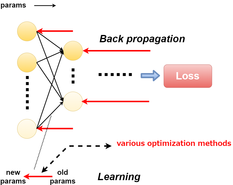
パラメーターを更新する方法を最適化関数で決めます。
The optimization function determines how to update the parameters.
今回のシリーズで採用している最適化の関数はAdamですよね〜。
The optimization function used in this series is "Adam".
微分
Differentiation
では趣旨を踏まえた上でBackpropagationの基礎の部分である微分について説明していきます。
I'll briefly describe differentiation that is the foundation of backpropagation based on the purport.
微分についてですが、大砲から玉を発射することを想像してくだちぃ。
First of all, I would like to explain differential calculus. imagine shooting balls from a cannon.
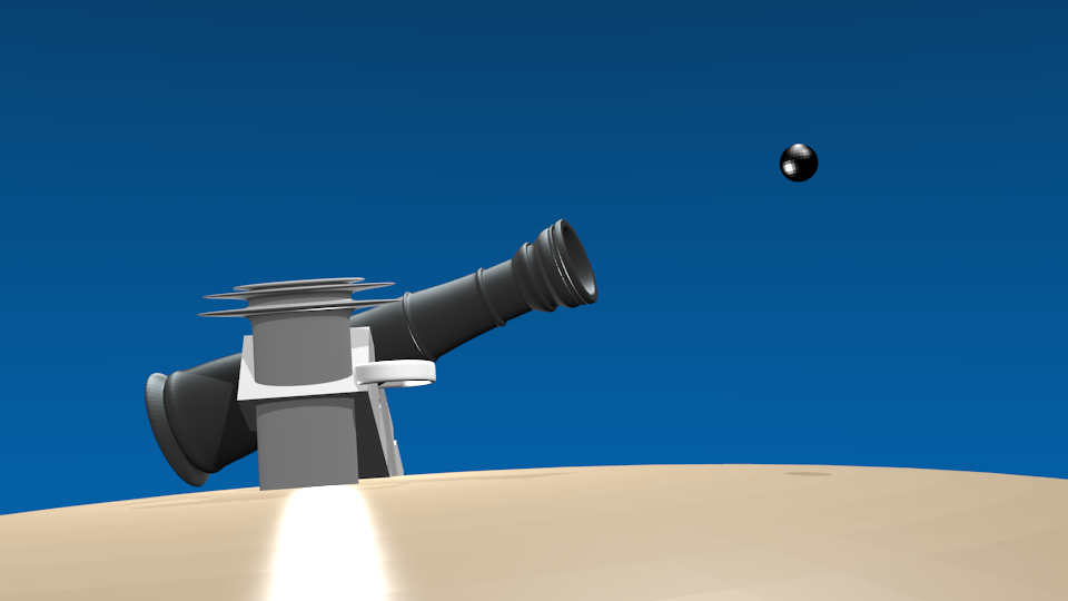
発射された玉の「平均時速」が毎秒750mだとしたら、単純計算で一秒間に進む距離は750メートルです。
If the "average speed" of a launched ball is 750 meters per second, a simple calculation shows that it will travels 750 meters in 1 second.
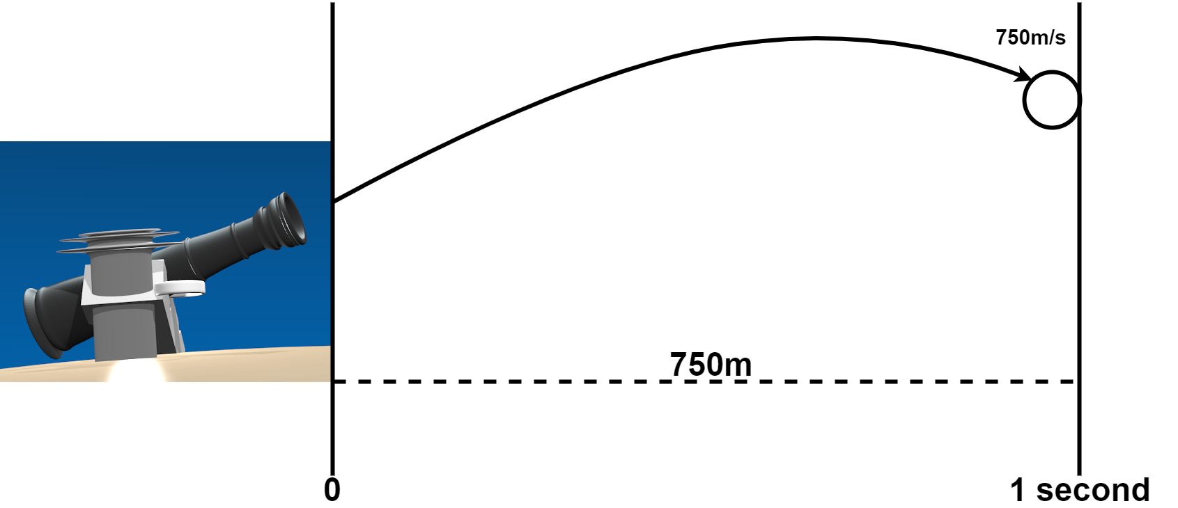
でも実際にはこれは「速度を平均化したものの結果です」です。空気抵抗や重力の影響で「瞬間的な」速度と進む距離は変わっていきます。
But in reality, this is "mean velocity". "momentary" velocity and travel distance are affected by air resistance and gravity.
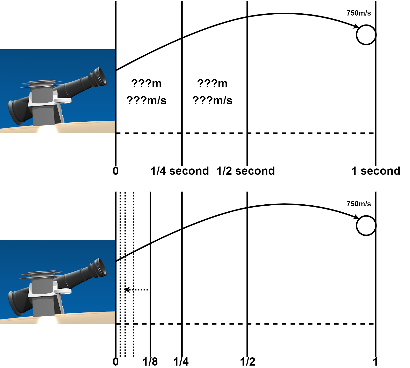
微分の考え方は、大砲の弾丸の軌道を細かく分割していって「瞬間的な数値」を計測することです。
The concept of differentiation is to measure "instantaneous numerical value" by subdividing the trajectory of a cannon ball.
微分の数式は以下です。
The formula for differentiation is below.
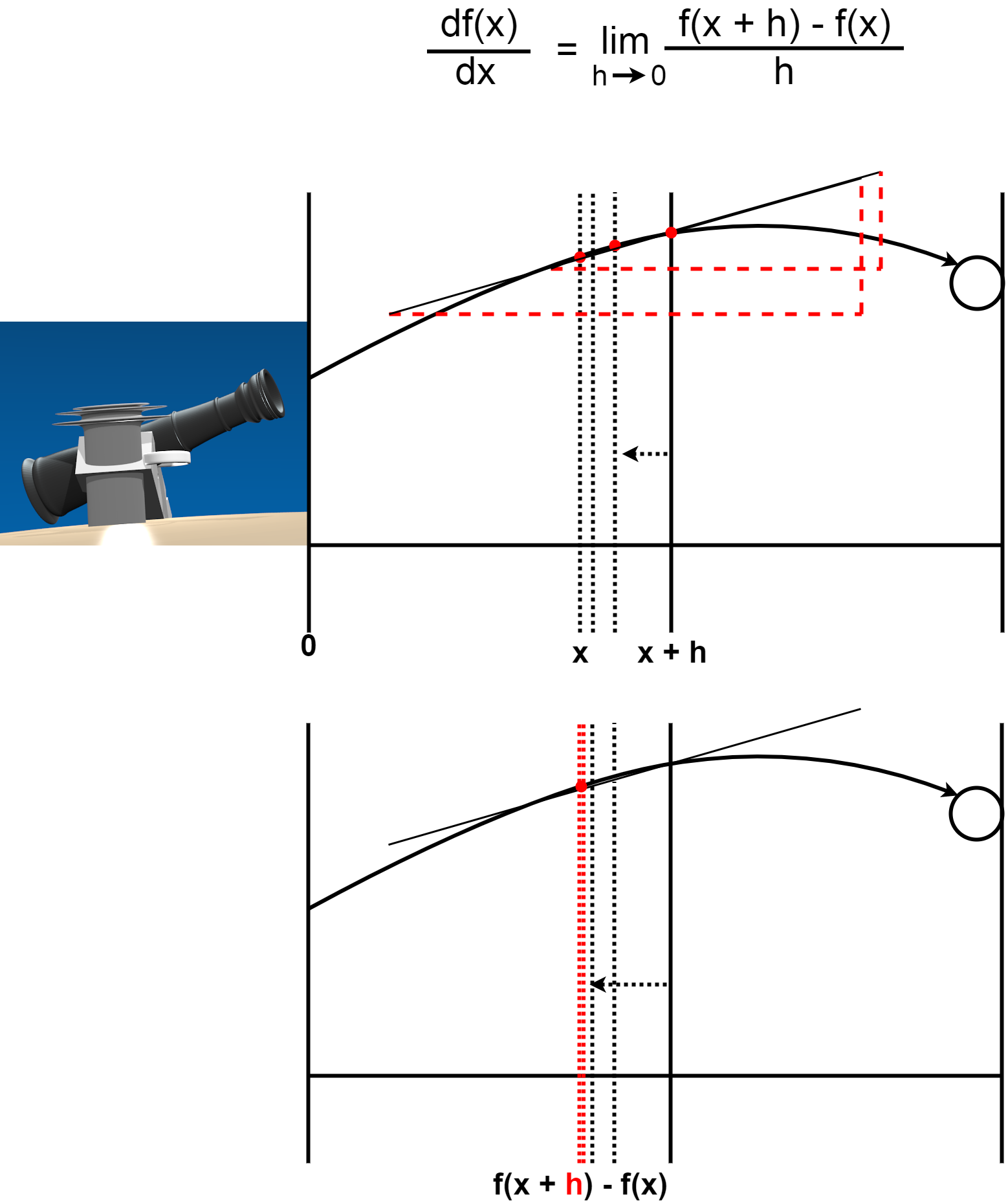
「h」は限りなくゼロに近い値。 「h」が限りなくゼロに近づけば、弾道におけるある点に接線が引くことができます。 その接線の傾きがゼロになった時、弾道の曲線は最大まで上昇したと考えることができます。
"h" is infinitely close to zero numerical value. If "h" approaches zero as close as possible, the tangent can be drawn to a point in the trajectory. When the slope of the tangent is zero, the trajectory curve can be considered to have risen to its maximum.
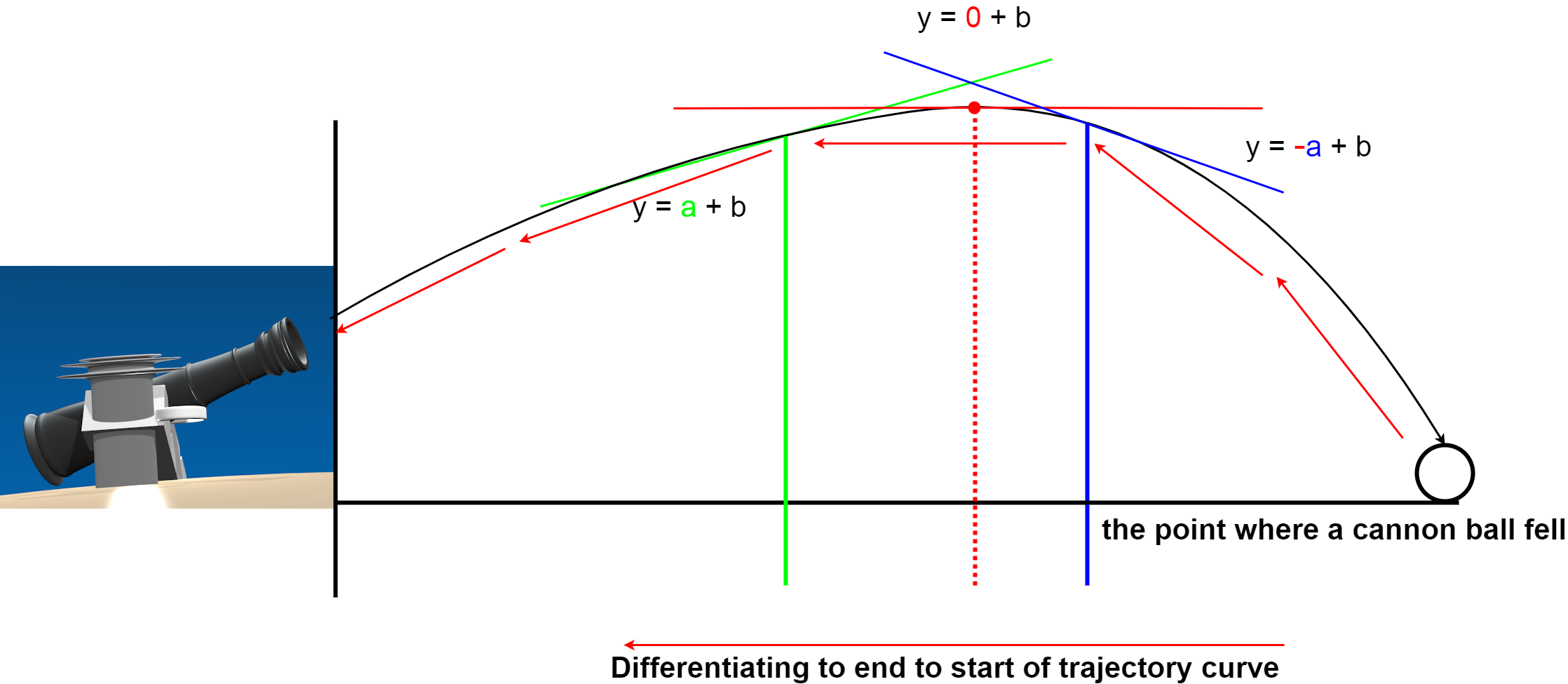
このように微分を使えば砲弾が落ちたポイントから、弾道を予測できて、次からは大砲の火薬や砲弾の重さ、大砲の角度を微調整することによって、ほぼ正確に目的地に命中させることが可能になります。
Thus, by using the differentiation, the trajectory can be predicted from the point where the cannon ball falls, and the next time, it is possible to hit the target without depending on the human sense almost accurately by finely adjusting the weight of the cannon, the quantity of gunpowder and the angle.
Pythonで微分
Differentiation using Python scripts
微分の大体の意味が分かったと思うので、ある関数(f(x))が図のような形になった時を考えてみませう。
Now that you have a general idea of the meaning of differentiation, let's apply it to the case when a function (f(x)) takes the form looks like this.
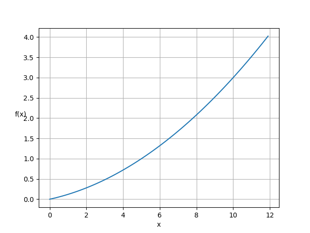
この図をPythonで書くとこうなります。
This is what the diagram looks like in Python.
import numpy as np
import matplotlib.pyplot as plt

def func(x):
  return 0.02 * x **2 + 0.1 * x

x = np.arange(0.0, 12.0, 0.1)
y = func(x)
plt.xlabel('x')
plt.ylabel('f(x)',  rotation=0)
plt.grid()
plt.plot(x, y)
plt.show()
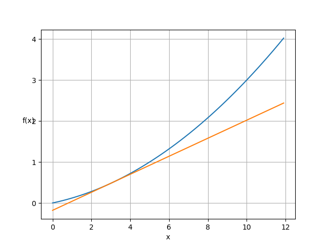
それでは微分をするPythonスクリプトを書きましょう。
Let's write a Python script that differentiates.
def differentiation(f,x):
    h = 1e-8
    return (f(x+h) - f(x-h)) / (2*h)
def tangent(f, x):
    d = differentiation(f,x)
    y = f(x) - d*x
    return lambda t: d*t + y
tf1 = tangent(func, 3.0)
y2 = tf1(x)
plt.xlabel('x')
plt.ylabel('f(x)',  rotation=0)
plt.grid()
plt.plot(x, y)
plt.plot(x, y2)
plt.show()
このように関数が描く曲線に対して接線を引くことができます。
You can see a tangent to the curve that the function draws.
少し遊んでみましょう。
Let's try various things.
tf1 = tangent(func, 3.0)
tf2 = tangent(func, 6.0)
tf3 = tangent(func, 9.0)
y2 = tf1(x)
y3 = tf2(x)
y4 = tf3(x)
plt.xlabel('x')
plt.ylabel('f(x)',  rotation=0)
plt.grid()
plt.plot(x, y)
plt.plot(x, y2)
plt.plot(x, y3)
plt.plot(x, y4)
plt.show()
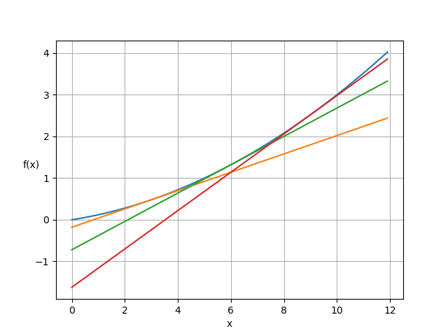
ごちゃごちゃしてて分かりにくいですが、ちゃんと接線が引けています。
It's cluttered and hard to see, but the tangents are drawn well.
残りの説明は次回に持ち越します。お次は微分から派生する勾配についての説明を予定してます。
I will carry over the rest of the explanation next time. Next, I'm going to explain the gradient related to the differentiation.