Tensorflowとは、Googleが提供しているオープンソースの機械学習用ライブラリですが、深層学習（Deep Learning）にも使われています。

Tensorflow is an open source machine learning library from Google Inc, but is also used for deep learning.

ということである程度簡単にTensorflowについて知っておきましょう。

So let's get to know about Tensorflow a bit more easily.

まず最初にTensorflowのTensorの意味ですが、簡単に説明しますと、以下の画像のようになります。

First of all, the meaning of Tensorflow's Tensor is as shown in the following image.

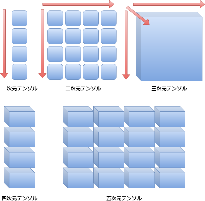
• ※ 「一次元」 means one-dimensional. 「テンソル」 means Tensor
• ※ 「二次元」 means two-dimensional.
• ※ 「三次元」 means three-dimensional.
• ※ 「四次元」 means four-dimensional.
• ※ 「五次元」 means five-dimensional.

このようにTensorflowで使われているTensor（テンソル）の意味とは、N（任意の数）次元の配列（ベクトル）のことです。

Thus, The meaning of Tensor (tensor) as used in Tensorflow is an array of N (any number) dimensions (Vector).

ちなみに、よく数学などで使われているスカラー、ベクトル、行列とかと、テンソルは以下のようになります。

By the way, scalar, vector, matrix and tensor which are often used in mathematics are as follows.

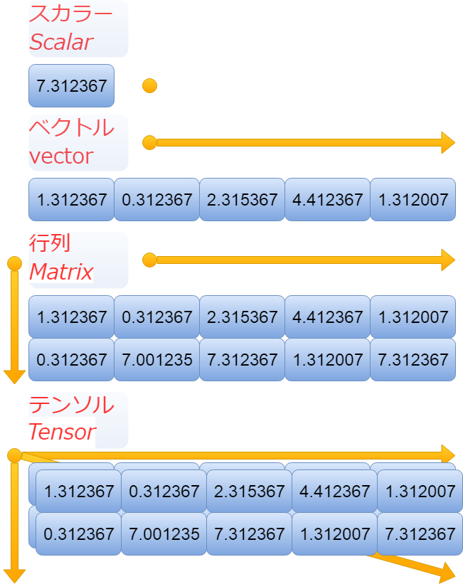
ちょっと混乱しますよね。 でも要するに、上の画像でのベクトルが一次元（一階）のテンソル。 行列が二次元（二階）のテンソルだと思ってもらえればいいかと。 単にテンソルが三次元（三階）以上のテンソルだと思ってもらえればいいかと。

It's a little confusing.But basically, the vector in the image above is a one-dimensional (first rank) tensor. Think of matrix as a two-dimensional (second rank) tensor. Think of it simply as a tensor that is more than three-dimensional (third rank).

それでも分かりにくい！そんな悩みを解決してくれる有り難いものがあります。 Pythonには計算用ライブラリのNumpyというものがあり、これを使えばコードを書きながら理解できます。 （小難しい理論があろうが、どのみちPythonのコードを書かなきゃ始まらないしね。）

It's still hard to understand. I am grateful that there is something that solves such a problem. Python has a computational library called Numpy that you can use to understand while writing code. (There's a little hard theory, but you have to write Python code anyway.)

それではNumpyをインポートしましょう。（無ければ pip install numpy）

Let's import Numpy. (If you don't have one, use [pip install numpy])

感謝の意を込めて、Numpyを別名Thank you Numpyでインポートします。。。

To thank Numpy, import it with the alias Thank you Numpy.

import numpy as thank_you_numpy
.............

すんまそん。普通にインポートします。

Sorry about that. Import normally.

import numpy as np

まず一次元のテンソル（ベクトル）は以下のようになります。 ここでNumpyのシェイプを使えば、次元数を見ることができます。 （一次元、二次元、三次元…）といった具合に。

First, the one-dimensional tensor (Vector) is. Using Numpy's shape, you can see the number of dimensions. Like, (One dimensional, two dimensional, three dimensional...).

ただ気をつけたいのは（３、４）このように表示されるので、 これは（三行四列の行列で、二次元のNumpy配列ですよ。）といった意味です。

The only thing I want to be careful about is that (3, 4) is displayed like this. It means (It's a three rows, four columns matrix, a two-dimensional Numpy array).

"""Numpy配列
Expressed in a Numpy array."""
In [3]: np.array([1,1,1])
Out[3]: array([1, 1, 1])
"""
一次元数
One dimensional count.
"""
In [4]: np.array([1,1,1]).shape
Out[4]: (3,)

一次元テンソル,この場合３つの数字の並び「1、1、1」のNumpy配列。要は単なるベクトルです。

A one-dimensional tensor, in this case a Numpy array of 3 digits [1, 1, 1]. It's just a vector.

続いての説明を一気にします。

Next, I will explain all at once.

"""Numpy配列
Expressed in a Numpy array."""
In [5]: np.array([[1,1,1],[1,1,1]])
Out[5]: 
array([[1, 1, 1],
       [1, 1, 1]])
"""
二次元数
Two dimensional count.
"""
In [6]: np.array([[1,1,1],[1,1,1]]).shape
Out[6]: (2, 3)

"""Numpy配列
Expressed in a Numpy array."""
In [7]: np.array([[[1,1,1],[1,1,1]],[[1,1,1],[1,1,1]]])
Out[7]: 
array([[[1, 1, 1],
        [1, 1, 1]],

       [[1, 1, 1],
        [1, 1, 1]]])
"""
三次元数
Three dimensional count.
"""
In [8]: np.array([[[1,1,1],[1,1,1]],[[1,1,1],[1,1,1]]]).shape
Out[8]: (2, 2, 3)

二次元配列はすぐ分かると思いますが、三次元がややこしいですね。

Two-dimensional arrays are easy to understand, but three-dimensional is complicated.

ですが、こう考えれば分かりやすいです。２行、３列の配列（行列）が２個並んだ配列（ベクトル）がある。（「２」（ベクトル）、「２行、３列」（行列））

But it is easy to understand if you think like this. There are 2 arrays (Vector) of 2 rows and 3 columns (matrix). (2 (Vector), 2 rows, 3 columns (matrix))

続いて四次元のNumpy配列も以下のように考えることができます。

The four-dimensional Numpy array can then be thought of as.

"""Numpy配列
Expressed in a Numpy array."""
In [9]: np.array([[[[1,1,1],[1,1,1]]],[[[1,1,1],[1,1,1]]]])
Out[9]: 
array([[[[1, 1, 1],
         [1, 1, 1]]],


       [[[1, 1, 1],
         [1, 1, 1]]]])
"""
四次元数
Three dimensional count.
"""
In [10]: np.array([[[[1,1,1],[1,1,1]]],[[[1,1,1],[1,1,1]]]]).shape
Out[10]: (2, 1, 2, 3)

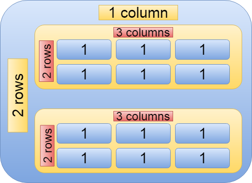
つまり、二行一列の行列の中身は二行三列の行列。

In other words, the contents of a matrix of two rows and one column are a matrix of two rows and three columns.

イメージとして考えると以下のようになります。

The image is as follows.

そして、テンソルはデータタイプという属性値があります。 文字か数値が入れられると考えれば簡単です。

And the tensor has an attribute value called data type. It's easy if you think you can put letters or numbers.

ですが、詳しくどんなタイプが入れられるかを説明していきます。

But I will explain in detail what types are available.

• Int型（整数）（１、２、３…）

• Data type is Int (Integer) (1, 2, 3...)

• Float型（小数）（1.1,  2.23,  3.89...）

• Float type (Decimal) (1.1,  2.23,  3.89...)

• Bool型（真理値）（True、False...）

• Bool type (truth value) (True, False...)

• String型（文字列など）（"猫"、"ネズミ"、"トムとジェリー"...）など。

• String type (String, etc.), such as ("Cat", "Mouse", "Tom and Jerry"...) etc.




文字列だけ若干ややこしいのでコードで説明。

The string itself is a bit confusing, so I will explain it in code.

• import tensorflow as tf
  import codecs
  
  text = tf.constant("トムとジェリー means Tom and Jerry.")
  
  text.dtype
  --> tf.string
  
  text.eval()
  --> b'\xe3\x83\x88\xe3\x83\xa0\xe3\x81\xa8\xe3\x82\xb8\xe3\x82\xa7\xe3\x83\xaa\xe3\x83\xbc means Tom and Jerry.'
  
  codecs.decode(text.eval(),encoding='utf-8')
  --> 'トムとジェリー means Tom and Jerry.'
  
  text_chars = tf.constant([ord(char) for char in u"トムとジェリー means Tom and Jerry."])
  
  text_chars.dtype
  --> tf,int32
  
  text_chars.eval()
  array([12488, 12512, 12392, 12472, 12455, 12522, 12540,    32,   109,
           101,    97,   110,   115,    32,    84,   111,   109,    32,
            97,   110,   100,    32,    74,   101,   114,   114,   121,
            46])
  # 12488 -> ト
  
  ''.join([codecs.decode(char,encoding="utf-32") for char in text_chars.eval()])
  --> 'トムとジェリー means Tom and Jerry.'
  

続いて、Graphですが、 これは所謂計算ノードグラフと言われているものと似ています。 図で説明すると以下になります。

Next is the Graph, which is similar to the so-called compute node graph. This is illustrated below.

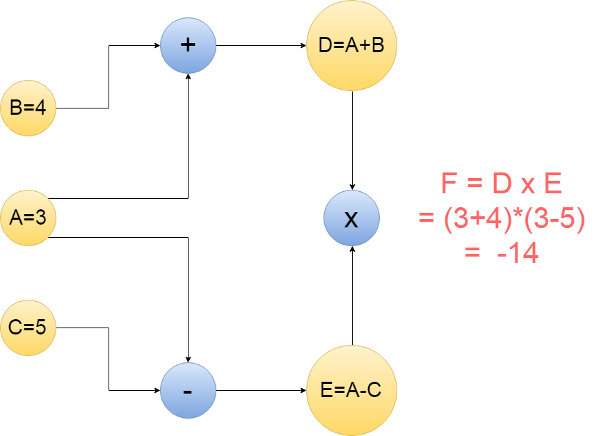
上の丸はノードと言われていて、矢印はエッジと言われています。 それぞれの意味の説明をすると、 「+」は矢印からきた数字を「足し算する」。 「-」は矢印からきた数字を「引き算する」。 「x」は矢印からきた数字を「掛け算する」。 もちろんノードには「平方根」や「自乗」も使える。 単純でしょ？

The top circle is called a node and the arrow is called an edge. A description of each meaning. 「+」 is the number from the arrow 「add」. 「-」 is the number from the arrow 「subtract」. 「x」 is the number from the arrow 「multiply」. Nodes can also be 「square root」 or 「square」, of course. Simple, right?

このような形にすることによって、ニューラルネットワークモデルや計算方法を組むことが分かりやすくなります。

This makes it easier to build neural network models and calculation methods.

実際に上の画像の計算式をTensorflowで組んでみましょう。

Let's actually create the formula in the above image using Tensorflow.

import tensorflow as tf
A = tf.constant(3)
B = tf.constant(4)
C = tf.constant(5)
D = tf.add(A,B)
E = tf.subtract(A,C)
F = tf.multiply(D, E)

これで計算グラフが出来上がりました。 続いて、一気にテンソル（矢印の数値）をフロー（計算が流れる）させるために、セッションということを行います。 セッションついての簡単な説明は以下の画像を見てください。

Now that We have a calculation graph, To make the tensor (number in the arrow) flow (Do the calculation in the flow work.) all at once, we have a session. A brief description of the session can be found in the image below.

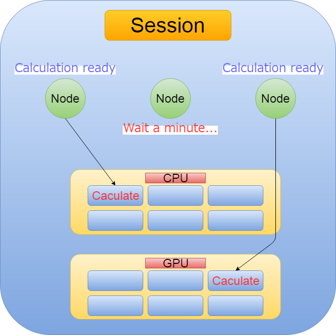
つまりSessionとは、 Tensorflowが計算可能になったノードを、 非同期/並列的にCPUやGPUなどに割り当てて計算を処理してくれること。

Session means that Tensorflow allocates computable nodes to the CPU or GPU asynchronously or in parallel to process the computation.

コードは以下になります。 With文は文の終わりで自動的にセッションをクローズしてくれます。

The code is as follows. The With statement automatically closes the session at the end of the context.

with tf.Session() as sess:
  result = sess.run(F)
  print(result)
--> -14

ある程度の概要が分かったところで、線形回帰モデルをTensorflowで作ってみましょう。

Now that you have some idea, let's build a linear regression model with Tensorflow.

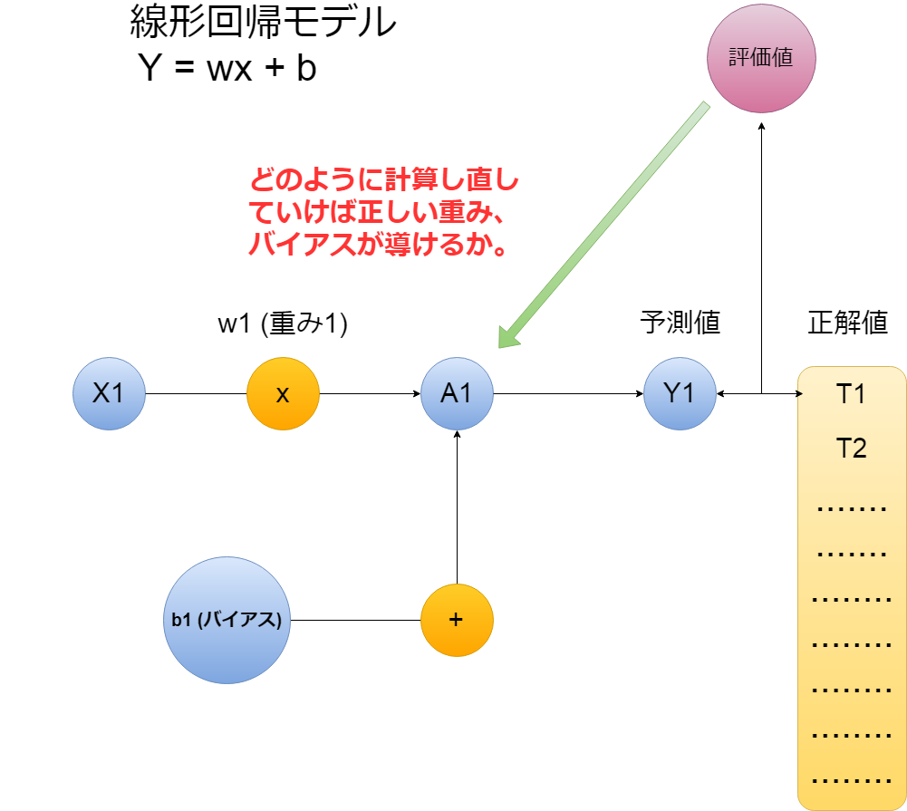
以下単純な線形回帰モデルです。

The following is a simple linear regression model.

下のコードに出てくる、 Placeholderとは、一度作ると後にどんな値でも入れられる便利な変数の宣言方法です。

In the code below, Placeholder is a convenient way to declare a variable that can be created once and then populated with any value.

import tensorflow as tf

# 重み、（傾きのようなもの）を初期値0.5として作ります。
# Weight (something like the slope of a straight line) with an initial value of 0.5.
w = tf.Variable([.5], tf.float32)

#バイアス、（切片のようなもの）を初期値-0.5として作ります。
# Bias (like the intercept of a linear equation) with an initial value of -0.5.
b = tf.Variable([-0.5], tf.float32)

# 入力値のXをプレースホルダーでどんな値が入ってもいいように作り置きします。
# Set the input value X as a placeholder so that any value can be entered.
x = tf.placeholder(tf.float32)

# 線形回帰の方程式を作ります。
# Create a linear regression equation.
linear_exp = x * w + b

# 全ての変数を初期化して、グラフを作り上げます。
# Initialize all variables and construct a graph.

# sessionを開始することによって、実際の計算が構築されたグラフによって行われ、
# 出力結果が確認できるようになります。
# By starting session, the actual computation is performed by the constructed graph and the output can be seen.
s = tf.Session()
i = tf.global_variables_initializer()
s.run(i)

# Xの値を１、２、３として計算してみます。
# Try calculating X as 1, 2, 3.
print(s.run(linear_exp,{x: [1,2,3]}))

# 表示
# to try to display
# => [0.  0.5 1. ]

実際の問題に使えるように、上のコードの変数をイメージしていきます。 上で作った「x」が「ある道路の一日の交通量」だったら。 「y」が「ある目的地までの自宅から自動車でかかる時間」だったら。

So that you can use it for real world data, imagine the variables in the code above. If the x you made above is "the daily volume of traffic on a road". If y is "the time it takes from home to a destination by car".

この「x」が特徴量で、目的変数が「y」になります。 以上を踏まえてもう一度コードを書いていきましょう。

This "x" is the Features and the Target variable is "y". So let's write the code again.

# Xの値を「自動車で通行した一定の時間の、交差点Aから交差点Bまでの交通量、自動車の数」だとします。
# Suppose the value of X is "the volume of traffic from intersection A to intersection B, and the number of motor vehicles in a car during a given period of time".
# 一日目を30台、次を25台というふうにxに入れていきます。
# Put 25 units on the 1st day, 30 units on the next day, and so on into x.

# 調べた数のリストを用意。
# Prepare a list of the numbers you checked.
traffic=[30, 25, 63, 39, 42, 50, 44, 25, 22, 47, 45, 73, 38, 77, 28, 48, 64,
98, 93, 82, 52, 36, 36, 78, 93, 59, 23, 83, 80, 88]

print(s.run(linear_exp,{x: traffic}))

# 表示
# to try to display
# これを単位「分」で読むとそれらしく見えませんか？
# If you read this in "minutes," doesn't it look like it?
# => [14.5 12.  31.  19.  20.5 24.5 21.5 12.  10.5 23.  22.  36.  18.5 38.
13.5 23.5 31.5 48.5 46.  40.5 25.5 17.5 17.5 38.5 46.  29.  11.  41.
39.5 43.5]

ここで正解データを用意して、予測した値とどれだけ剥離しているかを計算する必要があります。

You now need to have the correct data to calculate how much separation from the predicted values.

# 正解データとして、リストとプレースホルダーを用意する。
# Prepare lists and placeholders for correct data.
correct_data=[18.9, 11.7, 18. , 17.1, 14.4, 18.9, 15.3, 18. , 17.1, 16.2, 15.3,
14.4, 18.9, 13.5, 16.2, 10.8, 17.1, 16.2, 11.7, 13.5, 18.9, 11.7,
12.6, 18. , 18.9, 18. , 16.2, 10.8, 14.4, 13.5]
t=tf.placeholder(tf.float32)

# 精度評価指標に二乗平均平方根誤差（RMSE：Root Mean Squared Error）を使用します。
# Use Root Mean Squared Error as the accuracy evaluation index.
error=linear_exp-t
squared_errors=tf.square(error)
reduce_mean=tf.reduce_mean(squared_errors)
loss=tf.sqrt(reduce_mean)

# 予測値と正解値を比べてみます。
# Compare the predicted value with the correct value.
print(s.run(loss,{x:traffic,t:correct_data}))
# => 17.036636

L（損失） = root(平方根)（ 1/n（データの数） * sum（（yi（予測値） - ti（正解値））2(二乗) ）

L (loss) = root (square root) (1/n (Number of data) * sum ((yi (predicted value) -ti (correct value)) 2 (squared))

言葉や式でわかる通り、予測値と正解値の誤差が０になれば RMSEの値もゼロに近づきます。

As you can see from the words and expressions, if the error between the predicted value and the correct value becomes zero, RMSE also approaches zero.

極端な話、30個のXの値から30個のYが導かれ、 30個の正解データTとの誤差が全て0.1だったら？ もしくは全て10だったら？ 全て0.1のほうが上手く学習できてますよね。 これをRMSEで解くと

At the extreme, what if 30 Y's are derived from 30 X's, and the error with 30 correct data T is all 0.1? Or all 10? All 0.1 are better at learning. If you solve this with RMSE,

error1=np.array([0.1]*30)
error2=np.array([10]*30)
squared_errors1=np.square(error1)
squared_errors2=np.square(error2)
reduce_mean1=np.mean(squared_errors1)
reduce_mean2=np.mean(squared_errors2)
loss1=np.sqrt(reduce_mean1)
loss2=np.sqrt(reduce_mean2)

print(loss1)
# => 0.10000000000000002
print(loss2)
# => 10.0

これで直感的に分かったと思います。 ではどのようにして、損失値を下げていくか。

Now, I think you have an intuitive idea. So how do you reduce your losses?

そのためには、 損失値を見て、一つ前の計算に遡り、 微分をして、重みやバイアスを調整していきます。

To do this, look at the loss value, go back to the previous calculation, and adjust the weight and bias by differentiating.

ここで、その微分をして、パラメータを最適化するアルゴリズムに、 最急降下法（Gradient descent）があります。 これをTensorflowではOptimizer（最適化するもの）としてすでに用意してくれています。

Here, one algorithm for differentiating and optimizing parameters is the Gradient Descent method. Tensorflow already offers this as an Optimizer

最適化アルゴリズムとセットになっている学習率 これはどの程度の幅でXとYを微分するかだと思っていただければわかりやすいです。

The learning rate that comes with the optimization algorithm is easy to understand if you think of it as the differential width between X and Y.

大きければ、学習スピードは上がります。 しかし、その幅が大きいため最適解を見過ごしてしまいがちです。 逆に小さければ、学習コストは増大して、 CPUやGPUなどに負荷がかかります。 基本として、始めは学習率を大きめにとり、除々に下げていきます。

The bigger, the faster you learn. However, it is easy to overlook the optimal solution because of its wide range. On the other hand, if it is small, the learning cost will increase, and the CPU, GPU. will be burdened. Basically, you should start with a higher learning rate and gradually lower it.

図式したものはこの記事を見てください。

See this page for a diagram.

では実際に使っていきましょう。

Lets get started.

# 最適化アルゴリズムに最急降下法を指定して、
# 学習率（Learning rate)はに0.01設定します。
# Specify the Gradient descent method for the optimization algorithm, and set the Learning Rate to 0.01.
optimizer=tf.train.GradientDescentOptimizer(0.01)

# 損失値が最小になるようにトレーニングを開始する準備。
# Prepare to begin training to minimize loss values.

train=optimizer.minimize(loss)

# 1000回学習していきます。 
# We will learn 1000 times.
for i in range(1000):
  s.run(train,{x:traffic,t:correct_data})

# 更新されたパラメーターを見てみます。
# Look at the updated parameters.
print(s.run([w,b]))
# => [array([0.56360868], dtype=float32), array([0.981251], dtype=float32)]

# この重みとバイアスでどれぐらい改善されたか見てみます。
# Let's see how much this weight and bias improves it.
print(s.run(loss,{x:traffic,t:correct_data}))
# => 18.56

逆に結果が悪くなっています。

On the contrary, the result is worse.

ここで、学習率と学習回数を変えてみます。

Now, let's change the learning rate and number of times.

# 学習率を下げる
# Reduce the rate of learning
optimizer=tf.train.GradientDescentOptimizer(0.001)
print(s.run(loss,{x:traffic,t:correct_data}))
# => 18.05
# あまり変わらず。
# Not much.

# 学習率をもっと下げて、学習回数を多めにする
# Reduce the rate of learning and increase the number of learning
optimizer=tf.train.GradientDescentOptimizer(0.0001)
for i in range(10000):
  s.run(train,{x:traffic,t:correct_data})
print(s.run([w,b]))
# => [array([0.00506863], dtype=float32), array([15.025884], dtype=float32)]
print(s.run(loss,{x:traffic,t:correct_data}))
# => 2.6486938
# 大幅に改善されました。
# It has been greatly improved.

# ではもっと学習率を下げて、学習回数をあげたら？
# Why don't you lower the learning rate and increase the number of lessons?
# 学習率0.00001、学習回数100,000
# Learning rate : 0.00001
# number of learning : 100,000
optimizer=tf.train.GradientDescentOptimizer(0.00001)
for i in range(100000):
  s.run(train,{x:traffic,t:correct_data})
print(s.run([w,b]))
#=> [array([0.00360868], dtype=float32), array([15.121251], dtype=float32)]
print(s.run(loss,{x:traffic,t:correct_data}))
#=> 2.632239

# ではもっともっと学習率を下げて、学習回数をあげたら？
# Why don't you lower your learning rate and increase your learning rate?
# 学習率0.000001、学習回数1,000,000
# Learning rate : 0.000001
# number of learning : 1,000,000
optimizer=tf.train.GradientDescentOptimizer(0.000001)
for i in range(1000000):
  s.run(train,{x:traffic,t:correct_data})
print(s.run([w,b]))
#=> [array([0.00360771], dtype=float32), array([15.121251], dtype=float32)]
print(s.run(loss,{x:traffic,t:correct_data}))
#=> 2.632239
# 学習時間が異常に跳ね上がっただけで、損失値は微動だにしませんでしたね。
# The learning time just jumped abnormally and the loss value was not small.

使ったのは実際あるちゃんとしたデータではないので、 正しいパラメーターの調整ではありません。 たった30個のランダムに決めたデータに100万回学習させても ほとんど何も変わりません。 学習時間が増えるだけです。

The data you used isn't real, so it's not adjusting the correct parameters. If you take just 30 random bits of data and you teach them 1 million times, it doesn't make much difference. It only increases learning time.

このデータを画像のピクセル値をNumpy配列にしたり、 Uberなどが提供している、実際の移動時間などのデータに置き換えてみてください。

You can make this data into a Numpy array of image pixel values. Instead, you can use data like actual travel times provided by Uber.

今回はTensorflowを使った方法を紹介しましたが、他のライブラリKerasや、Numpy等を使ってイチから組み立てても考え方や方法は変わりません。 最適化のアルゴリズムやニューラルネットワークの中間層を工夫する、パラメータの微調整、特徴量選択などを繰り返して、正しい学習モデルを作ることができます。

I've shown you how to do this with Tensorflow, but you can build it from scratch with other libraries like Keras or Numpy. It is possible to create a correct learning model by repeating the optimization algorithm, the intermediate layer of the neural network, the fine adjustment of the parameter, and the feature quantity selection.

基本的にTensorflowの学習スタイルはGraph計算ネットワークを駆使して、予測値と正解値を近づけるために最適化手法を使い、パラメータを更新して、入力に対して、正解に近い出力を出せる学習モデルを作ることです。

Basically, the Tensorflow learning style uses the Graph calculation network to create a learning model that uses optimization techniques to approximate predicted and correct values, updates parameters, and produces output that is close to correct for input.

Tensorflowは煩わしい、ニューラルネットワーク構築、最適化アルゴリズム などをできるだけ短いコードで書けるように開発されました。 これを機会に是非Tensorflowの公式チュートリアルなどをみて 練習をしてみてください。

Tensorflow is designed to write cumbersome neural network construction and optimization algorithms in as little code as possible. Take this opportunity to check out the official Tensorflow tutorials, etc.Please practice.

と、上から目線ですが、自分も完全なる初学者ですので、共に学んでいきましょう。

I said it from above, but I am also a complete beginner, so let's learn together.

ま、散々Chainerがいい！とか言ってきたんですが、TPUが使いたいので、Tensorflowも真面目に取り組まないとねっていう下心ですけど。

The real story is that I've been saying that Chainer is good, but I just want to use TPU, so Tensorflow has to be serious about it.

長々とお付き合い頂きありがとうございます。

Thank you for reading this long blog.